Building a QAOA implementation in Jasp#
In this tutorial, we will explain step-by-step how to build a custom QAOA implementation in Jasp for the example of the MaxCut problem.
First, let us recall the problem description for MaxCut:
Given a Graph \(G = (V,E)\) find a bipartition \(S\), \(V\setminus S\) of the set of vertices \(V\) such that the number of edges between \(S\) and \(V\setminus S\) is maximal.
For a graph \(G\) with \(n\) nodes, such a bipartition can be encoded with a QuantumVariable with \(n\) qubits: we measure the \(i\)-th qubit in 0 if the node \(i\) is in the set \(S\), and 1 if the node \(i\) is in the set \(V\setminus S\). The cut value is the number of edges \(e=(i,j)\) in \(G\) such that \(i\in S\) and \(j\in V\setminus S\).
In Jasp, varibales are decoded to integers (i.e. jax.numpy.int) and not to binrary strings. In this case, the binary representation of an integer encodes a bipartition of the graph \(G\). Therefore, repeated sampling from a QuantumVariable in a superposition state will result in an array of integers representing bipartitions of the graph \(G\). Within QAOA, we require a post processing function to compute the average cut value for an array of samples.
As a first step, we will learn how to write a post_processor that can be compiled using jax.jit into a highly optimized version using Just-In-Time (JIT) compilation. This can significantly speed up the execution of numerical computations.
Computing the Average Cut of a Graph with JAX#
Step 1: Import Libraries
First, we need to import the necessary libraries.
[1]:
import jax.numpy as jnp
from jax import jit, vmap
import networkx as nx

from qrisp import QuantumVariable, h, rx, rzz
from qrisp.jasp import sample, minimize, jaspify, jrange, make_jaspr
Step 2: Define the Function to Extract Boolean Digits
We will define a function that extracts the value of a specific bit (digit) from an integer.
[2]:
@jit
def extract_boolean_digit(integer, digit):
    return (integer >> digit) & 1
Step 3: Create the Cut Computer Function
The cut computer function calculates the cut value for a given integer representation of a bipartition of a graph. This function will use the edges of the graph to determine how many edges cross the cut.
[3]:
def create_cut_computer(G):
    edge_list = jnp.array(G.edges())  # Convert edge list to JAX array

    @jit
    def cut_computer(x):
        x_uint = jnp.uint32(x)
        bools = extract_boolean_digit(x_uint, edge_list[:, 0]) != extract_boolean_digit(
            x_uint, edge_list[:, 1]
        )
        cut = jnp.sum(bools)  # Count the number of edges crossing the cut
        return -cut

    return cut_computer
Step 4: Create the Sample Array Post Processor
This function will process an array of samples and compute the average cut using the cut_computer function. It will utilize JAX’s vectorization capabilities for efficiency.
[4]:
def create_sample_array_post_processor(G):
    cut_computer = create_cut_computer(G)

    def post_processor(sample_array):
        # Use vmap for automatic vectorization
        cut_values = vmap(cut_computer)(sample_array)
        average_cut = jnp.mean(cut_values)  # Directly compute average
        return average_cut

    return post_processor
Step 5: Example Usage
Now we can create a graph and use our functions to compute the average cut.
[5]:
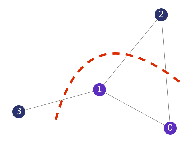
# Create a sample graph
G = nx.Graph()
G.add_edges_from([(0, 1), (1, 2), (2, 0), (1, 3)])

# Create the post processor function
post_processor = create_sample_array_post_processor(G)

# Sample input array representing different cuts
sample_array = jnp.array(
    [0b0001, 0b0010, 0b0100, 0b1000]
)  # Example binary representations

# Compute the average cut
average_cut = post_processor(sample_array)
print("Average Cut:", average_cut)
Average Cut: -2.0
So far, we created a function using JAX to compute the average cut of a graph efficiently. We defined a few helper functions, including one for extracting bits and another for calculating cuts, and then used JAX’s vectorization capabilities to process multiple samples effectively.
Setting up the QAOA#
For additional details, we refer to the QAOA tutorial.
Step 6: Define the QAOA ansatz
First, we will define the the cost operator and mixer.
[6]:
def create_cost_operator(G):

    def apply_cost_operator(qv, gamma):
        for pair in list(G.edges()):
            rzz(gamma, qv[pair[0]], qv[pair[1]])

    return apply_cost_operator


def apply_mixer(qv, beta):
    rx(beta, qv)
Next, we define the QAOA ansatz that creates a QuantumVariable, brings it into uniform superposition and applies \(p\) layers of the parametrized cost operator and mixer.
[7]:
def create_ansatz(G):

    apply_cost_operator = create_cost_operator(G)

    def ansatz(theta, p):
        qv = QuantumVariable(G.number_of_nodes())

        # Prepare uniform superposition
        h(qv)

        for i in jrange(p):
            apply_cost_operator(qv, theta[i])
            apply_mixer(qv, theta[p + i])

        return qv

    return ansatz
Step 7: Define the Objective Function
The objective function samples from the parametrized QAOA ansatz and computes the average cut value.
[8]:
def create_objective(G):

    ansatz = create_ansatz(G)
    post_processor = create_sample_array_post_processor(G)

    def objective(theta, p):

        res_sample = sample(ansatz, shots=1000)(theta, p)

        value = post_processor(res_sample)

        return value

    return objective
Step 8: Use a JAX-traceable Optimization Routine
We define the qaoa function for finding the optimal parameter values using the JAX-traceable minimize routine. It returns an array of optimal parameters and the average cost value for the optimal solution.
[9]:
def qaoa():

    # Create a sample graph
    G = nx.Graph()
    G.add_edges_from([(0, 1), (1, 2), (2, 0), (1, 3)])

    ansatz = create_ansatz(G)
    objective = create_objective(G)

    # Number of layers
    p = 3

    # Initial point for theta
    x0 = jnp.array([0.5] * 2 * p)

    result = minimize(objective, x0, (p,))

    # Sample from ansatz state for optimal parameters
    samples = sample(ansatz, shots=10)(result.x, p)

    return samples
Step 9: Run the QAOA
Finally, the jaspify method allows for running Jasp-traceable functions using the integrated Qrisp simulator. For hybrid algorithms like QAOA and VQE that rely on calculating expectation values based on sampling, the terminal_sampling feature significantly speeds up the simulation: samples are drawn from the state vector instead of performing repeated simulation and measurement of the quantum circuits.
[10]:
jaspify(qaoa, terminal_sampling=True)()
[10]:
array([ 9, 14, 10, 11, 3, 3, 12, 5, 5, 5])
You can also create the jaspr object and compile to QIR using Catalyst.
[ ]:
jaspr = make_jaspr(qaoa)()
qir_str = jaspr.to_qir()