qrisp.quantum_backtracking.QuantumBacktrackingTree.visualize_statevector

QuantumBacktrackingTree.visualize_statevector(pos=None, ax=None)

Visualizes the statevector graph.

Parameters:

posdict, optional

A dictionary indicating the positional layout of the nodes. For more information visit this page By default is suitable will be generated.

axmatplotlib.axes.Axes, optional

The axes object to draw the plot onto. If None, the current active axes is used. This is useful for creating grids of plots using plt.subplots.

Examples

We initialize a backtracking tree and visualize:

from qrisp import auto_uncompute, QuantumBool, QuantumFloat
from qrisp.quantum_backtracking import QuantumBacktrackingTree
import matplotlib.pyplot as plt

@auto_uncompute
def reject(tree):
    return QuantumBool()

@auto_uncompute
def accept(tree):
    return (tree.branch_qa[0] == 1) & (tree.branch_qa[1] == 1) & (tree.branch_qa[2] == 1)

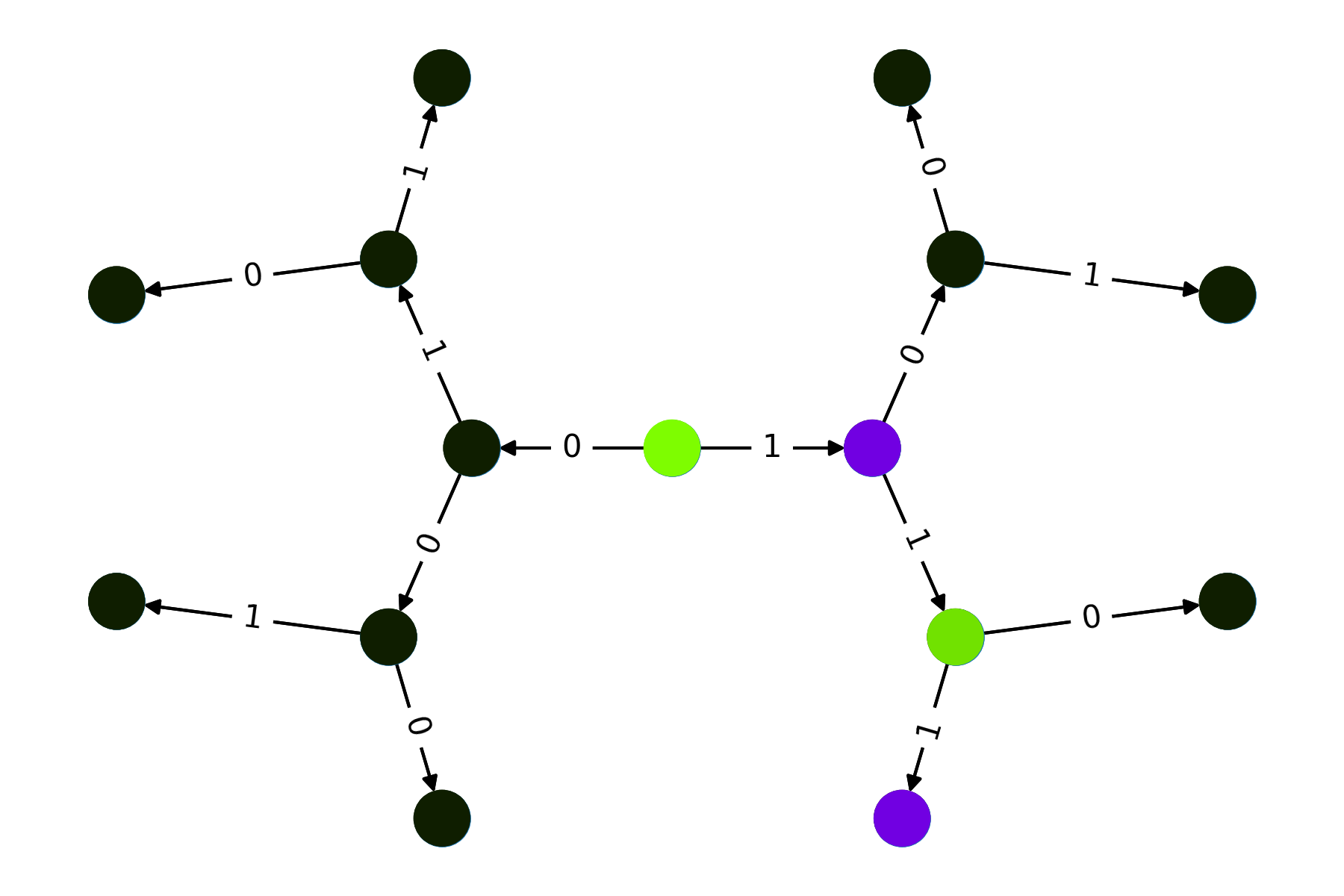
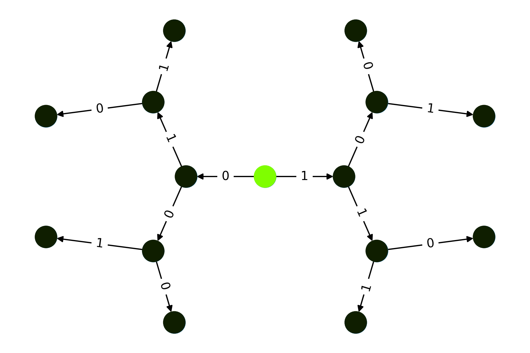
>>> tree = QuantumBacktrackingTree(3, QuantumFloat(1, name = "branch_qf*"), accept, reject)
>>> tree.init_node([])
>>> tree.visualize_statevector()
>>> plt.show()

>>> tree = tree.copy()
>>> tree.init_phi([1,1,1])
>>> tree.visualize_statevector()