Diagonal Hamiltonian Application

In the following example we will demonstrate how to compile arbitrary diagonal hamiltonians.

>>> import numpy as np
>>> import matplotlib.pyplot as plt
>>> from qrisp import QuantumFloat, QuantumChar, h, QFT, as_hamiltonian, multi_measurement

Hamiltonian function

We begin by specifiying a hamiltonian. This is achieved through a Python function that recieves elements form the labels of the QuantumVariable we would like to process and returns a value which represents the phase. In this case we are handling a QuantumFloat, so the input is a float. Another case could be where we are handling a QuantumChar, which implies that the hamiltonian function should be able to process characters.

def hamiltonian(x):

    return np.pi*np.sin(x**2*np.pi*2)*x

QuantumFloat example

We now create a QuantumFloat and bring it into uniform superposition. After that the hamiltonian function is applied.

>>> qf = QuantumFloat(5, -5, signed = True)
>>> h(qf)

To apply the hamiltonian, we call the app_phase_function method.

>>> qf.app_phase_function(hamiltonian)

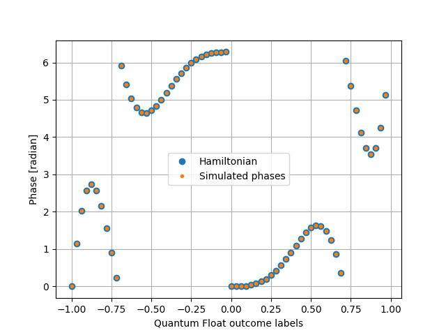
To visualize the results we retrieve the statevector as a function and determine the phase of each entry.

>>> sv_function = qf.qs.statevector("function")

This function receives a dictionary of QuantumVariables specifiying the desired label constellation and returns it’s complex amplitude.

Prepare the numpy arrays for plotting:

>>> x = np.array([qf.decoder(i) for i in range(2 ** qf.size)])
>>> sv_phase_array = np.angle([sv_function({qf : i}) for i in x])

Plot results

>>> plt.plot(x , hamiltonian(x)%(2*np.pi), "o", label = "Hamiltonian")
>>> plt.plot(x , sv_phase_array%(2*np.pi), ".", label = "Simulated phases")
>>> plt.ylabel("Phase [radian]")
>>> plt.xlabel("Quantum Float outcome labels")
>>> plt.grid()
>>> plt.legend()
>>> plt.show()

Multiple Arguments

In this example we will demonstrate how a phase function with multiple arguments can be synthesized. For this we will create a hamiltonian which encodes the fourier transform of different integers on the QuantumFloat qf conditioned on the value of a QuantumChar qch. We will then apply the inverse Fourier transform to qf and measure the results.

Defining the QuantumFloat qf as well as the QuantumChar c.

>>> qf = QuantumFloat(3)
>>> qch = QuantumChar()

Bring qf into uniform superposition so the phase function application yields a fourier transformed computation basis state. Afterwards bring qch into partial superposition (here \(\ket{a} + \ket{b} +\ket{c} +\ket{d}\)).

>>> h(qf)
>>> h(qch[0])
>>> h(qch[1])

In order to define the hamiltonian, we can use regular Python syntax. The decorator as_hamiltonian turns it into a function that takes Quantum Variables as arguments. The decorator will add the keyword argument t to the function which mimics the t in \(\text{exp}(i\text{H}t)\).

@as_hamiltonian
def apply_multi_var_hamiltonian(x, c):
    if c == "a":
        k = 2
    elif c == "b":
        k = 2
    elif c == "c":
        k = 3
    else:
        k = 4

    #Return phase value
    #This is the phase distribution of the Fourier-transform
    #of the computational basis state |k>
    return k*x*2*np.pi/2**qf.size

Apply Hamiltonian and inverse Fourier transform.

>>> apply_multi_var_hamiltonian(qf, qch, t = 1)
>>> QFT(qf, inv = True)

Acquire measurement results.

>>> print(multi_measurement([qch, qf]))
{('a', 2): 0.25, ('b', 2): 0.25, ('c', 3): 0.25, ('d', 4): 0.25}

Visualize the QuantumSession of the QuantumFloat qf.

>>> print(qf.qs)

QuantumCircuit:
--------------
       ┌───┐┌─────────────────────┐┌─────────┐
 qf.0: ┤ H ├┤0                    ├┤0        ├
       ├───┤│                     ││         │
 qf.1: ┤ H ├┤1                    ├┤1 QFT_dg ├
       ├───┤│                     ││         │
 qf.2: ┤ H ├┤2                    ├┤2        ├
       ├───┤│                     │└─────────┘
qch.0: ┤ H ├┤3                    ├───────────
       ├───┤│  app_phase_function │
qch.1: ┤ H ├┤4                    ├───────────
       └───┘│                     │
qch.2: ─────┤5                    ├───────────
            │                     │
qch.3: ─────┤6                    ├───────────
            │                     │
qch.4: ─────┤7                    ├───────────
            └─────────────────────┘
Live QuantumVariables:
---------------------
QuantumFloat qf
QuantumChar qch