qrisp.gqsp.dalzell_inversion#

dalzell_inversion(A: BlockEncoding, prep_b: Callable, t: float, eps: float, kappa: float) → BlockEncoding[source]#

Performs the Dalzell quantum algorithm to solve the Quantum Linear System Problem (QSLP) \(A\vec{x}=\vec{b}\), using kernel reflection. When applied to a state \(\ket{0}\), the algorithm prepares a state \(\tilde{x}\propto A^{-1}\ket{b}\) within target precision \(\epsilon\) of the ideal solution \(\ket{x}\). See also Dalzell’s talk for more details.

Warning

The returned BlockEncoding must be applied to operands in state \(\ket{0}\) (and not in state \(\ket{b}\)).

Instead of solving the system \(Ax=b\) directly, we consider the augmented system \(A_t x_t = b'\), i.e.,

\[\begin{split}A_t = \begin{pmatrix} A & 0 \\ 0 & t^{-1} \end{pmatrix} \begin{pmatrix} x \\ t \end{pmatrix} = \begin{pmatrix} b \\ 1 \end{pmatrix} = b'\end{split}\]

Equivalently, we can write the augmented system as \(A\ket{x_t}=\ket{b'}\) where

\[\begin{split}A_t = \ket{0}_a\bra{0}_a \otimes A + t^{-1} \ket{1}_a\bra{1}_a \otimes \ket{0}_s\bra{0}_s,\\ \ket{b'} \propto \ket{0}_a\ket{b}_s + \ket{1}_a\ket{0}_s, \quad \ket{x_t} \propto \|x\|_2\ket{0}_a\ket{x}_s + t\ket{1}_a\ket{0}_s\end{split}\]

Here, \(\ket{\cdot}_a\) denotes the state of the (1-qubit) ancilla variable, and \(\ket{\cdot}_s\) denotes the state of the system variable.

If \(A_t x_t = b'\), then

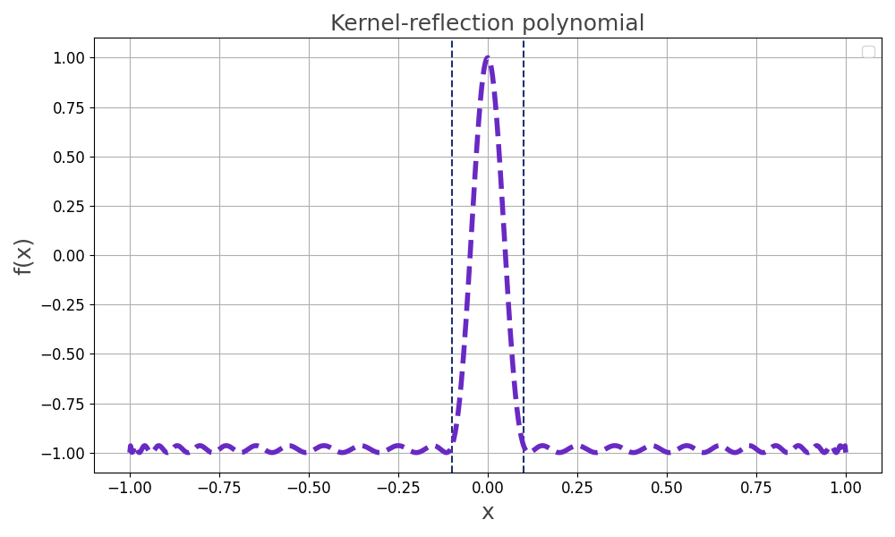
\[G_tx_t=(\mathbb{I} - \ket{b'}\bra{b'})A_t x_t = (\mathbb{I} - \ket{b'}\bra{b'})\ket{b'} = 0\]

Hence, the solution state \(\ket{x_t}\) is a kernel state (sigular value 0) of the operator \(G_t=(\mathbb{I} - \ket{b'}\bra{b'})A_t\). The kernel reflection operator \(K(G_t)\) reflects about the solution state \(\ket{x_t}\) to the augmented system, and can be implemented via QSVT using a polynomial approximation of the kernel reflection function \(K(\sigma)\colon [0,1] \to [-1,1]\) which maps the sigular value 0 to 1 and all other singular values to -1.

The algorithm consists of the following steps:

Introduce extra basis state \(\ket{e_n}=\ket{1}_a\ket{0}_s\) and prepare it as the initial state.
Choose \(t\simeq \|x\|_2\) and form the augmented linear system \(A_tx_t=b'\).
Apply the kernel reflection operator \(K(G_t)\), which reflects about the solution state to the augmented system.
Project the resulting state onto the \(\ket{0}_a\) subspace to obtain \(\ket{x}\).

The projection step can be implemented by post-selecting on the ancilla qubit being in state \(\ket{0}\) after applying the kernel reflection. The success probability of the algorithm depends on the choice of \(t\). If \(t\) is chosen to be on the order of \(\|x\|_2\), the algorithm succeeds with constant probability and only requires a constant number of repetitions.

../../../_images/chebyshev_kernel_reflection.png

Parameters:

ABlockEncoding: The block-encoded matrix to be inverted. It is assumed that the eigenvalues of \(A/\alpha\) lie within \(D_{\kappa} = [-1, -1/\kappa] \cup [1/\kappa, 1]\).
prep_bCallable: A function prep_b(*operands) preparing the right hand side \(\ket{b}\).
tfloat: An estimate \(t\) for the norm \(\|x\|_2=\|(A/\alpha)^{-1}b\|_2\) for normalized \(\|b\|_2=1\). The success probability depends on the the ratio \(t/\|x\|_2\). The optimal choice is \(t=\|x\|_2\). The estimate must lie in the interval \([1, \kappa]\). See below for more details.
epsfloat: The target precision \(\epsilon\).
kappafloat: An upper bound for the condition number \(\kappa\) of \(A\). This value defines the “gap” around zero such that all sigular values (eigenvalues) of \(A/\alpha\) lie in the domain \(D_{\kappa}\).

Returns:

BlockEncoding: A new BlockEncoding instance representing the kernel reflection operator.

Notes

Complexity: The query complexitiy of the algorithm is determined by the polynomial degree and scales as \(\mathcal O(\kappa\log(1/\epsilon))\). The success probability of the algorithm depends on the choice of \(t\) relative to \(\|x\|_2\):
- If the norm is known up to a constant factor, the algorithm succeeds with constant probability, hence only requires a constant number of repetitions.
- If the norm is unknown, methods for norm estimation can be used to find a suitable \(t\) with only a logarithmic overhead in the overall complexity.
For further insights, see Constant Factor Analysis of Optimal Quantum Linear Solvers in Practice, and make sure to use .resources() to compare the resources of different inversion methods in practice.
The polynomial is applied to operator \(G_t=(\mathbb I - \ket{b'}\bra{b'})A_t\). Each application of \(G_t\) requires 1 call to the block-encoding oracle for \(A\) and 2 calls to the state preparation oracle for \(b\). Hence, in contrast to other inversion() methods that only prepare the initial state once, the overall circuit complexity scales multiplicatively with the complexity of the state preparation oracle.

Examples

import numpy as np

A = np.array([[ 0.78, -0.01, -0.16, -0.1 ],
    [-0.01,  0.57, -0.03,  0.08],
    [-0.16, -0.03,  0.69, -0.15],
    [-0.1 ,  0.08, -0.15,  0.88]])

b = np.array([1, 1, 1, 1])

kappa = np.linalg.cond(A)
print("Condition number of A: ", kappa)
# Condition number of A:  2.020268873491503

from qrisp import *
from qrisp.block_encodings import BlockEncoding
from qrisp.gqsp import dalzell_inversion

BA = BlockEncoding.from_array(A)

def prep_b(operand):
    prepare(operand, b)

BA_inv = dalzell_inversion(BA, prep_b, 2.0, 0.01, 3.0)

@terminal_sampling
def main():
    # Prepare operand variable in state |0>
    operand = QuantumFloat(2)
    ancillas = BA_inv.apply(operand)
    return operand, *ancillas

res_dict = main()

# Post-selection on ancillas being in |0> state
filtered_dict = {k[0]: p for k, p in res_dict.items() \
                if all(x == 0 for x in k[1:])}
success_prob = sum(filtered_dict.values())
print("Success probability:", success_prob)
filtered_dict = {k: p / success_prob for k, p in filtered_dict.items()}

amps = np.sqrt([filtered_dict.get(i, 0) for i in range(len(b))])

c = (np.linalg.inv(A) @ b) / np.linalg.norm(np.linalg.inv(A) @ b)

print("QUANTUM SIMULATION\n", amps, "\nCLASSICAL SOLUTION\n", c)
# QUANTUM SIMULATION
# [0.51718522 0.43564501 0.60746181 0.41680095] 
# CLASSICAL SOLUTION
# [0.51643917 0.4380885  0.60597747 0.41732523]

Alternatively, use apply_rus to directly obtain the solution state without post-selection:

@terminal_sampling
def main():
    operand = BA_inv.apply_rus(lambda: QuantumFloat(2))()
    return operand

res_dict = main()
amps = np.sqrt([res_dict.get(i, 0) for i in range(len(b))])
print(amps)
# [0.51816163 0.43295659 0.60721322 0.4187472 ]